
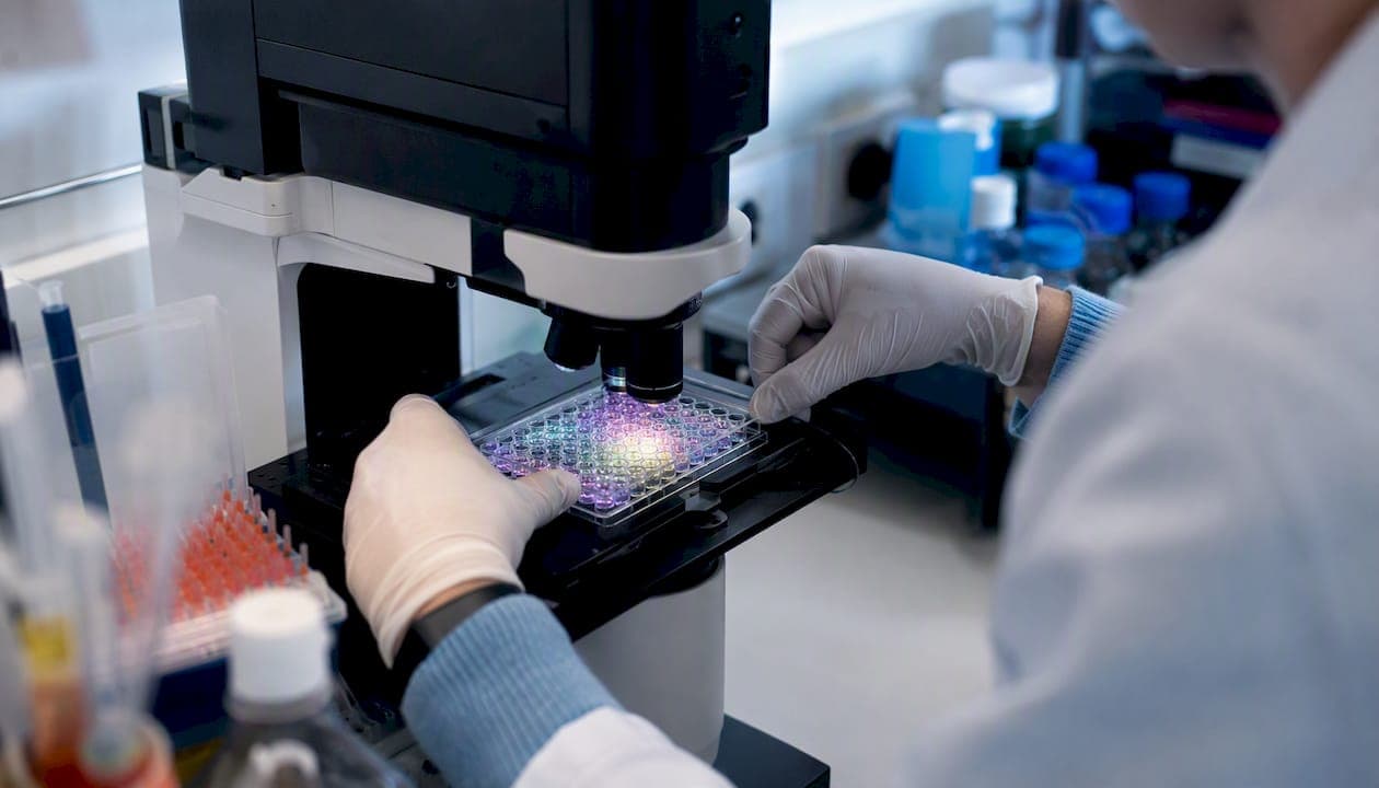
Cell Painting assays label six fluorescent dyes across five imaging channels to capture over 1,000 morphological features per cell, turning a standard microscopy plate into a high-dimensional readout of cell state. That single number is the reason this method has become a default choice for mechanism-of-action work, toxicity triage, and phenotypic screening.
A few things you need to know before committing lab time to it:
- Core biology captured: eight cellular compartments (nucleus, endoplasmic reticulum, nucleoli/RNA, actin cytoskeleton, Golgi, plasma membrane, mitochondria, and cytoplasm) via six stains.
- Output scale: typically 1,000 to 1,500 quantitative features per single cell, covering shape, texture, intensity, and spatial relationships.
- Timeline for a standard batch: roughly one to two weeks for culture, treatment, staining, and imaging, plus another one to two weeks for feature extraction and analysis on a batch of 20 plates or fewer.
- Primary applications: mechanism-of-action deconvolution, compound toxicity screening, and phenotypic clustering of chemical or genetic perturbations.
The canonical protocol from Bray et al., published in Nature Protocols, established the staining and imaging steps most labs still follow today, and a 2023 update refined stain concentrations for cost and reproducibility. If your project needs a morphological fingerprint of cell state rather than a single biochemical readout, this is very likely the right assay family. If you need a yes/no viability answer, it's overkill.
Key Takeaways
Reproducible Cell Painting results depend on rigorous imaging QC, validated stain concentrations, and batch-correction planning built in from the very first pilot plate, not added afterward.
| Point | Details |
|---|---|
| Follow published stain concentrations | Use v3-optimized concentrations from Nature Protocols rather than vendor-specific defaults. |
| Budget analysis time equally | Plan one to two weeks for feature extraction and QC alongside one to two weeks for wet-lab work. |
| Build controls into every plate | Include intra-plate and inter-plate replicates plus positive and negative controls from the pilot stage. |
| Match analysis method to dataset size | Use classical CellProfiler features for small studies; consider deep-learning embeddings at larger scale. |
| Partner out for rare-disease programs | Hopeatrarelabs integrates patient-derived iPSC modeling with morphological profiling and repurposed drug screening for ultra-rare disease projects. |
Table of Contents
- What Cell Painting Assays Actually Measure
- Cell Painting Protocol: A Stepwise Workflow
- Key Stains and Reagents for Cell Painting
- Imaging Setup and Throughput for High-Content Screening
- From Images to Data: The Cell Painting Analysis Pipeline
- Designing Robust Cell Painting Experiments
- Where Cell Painting Assays Deliver the Most Value
- Applying Cell Painting to Rare-Disease Modeling
- Where to Find the Protocols, Datasets, and Tools
- What Labs Get Wrong Starting Out
- How Hopeatrarelabs Applies Cell Painting to Rare Disease Programs
- Primary Sources and Recommended Reading
- Sources
What Cell Painting Assays Actually Measure
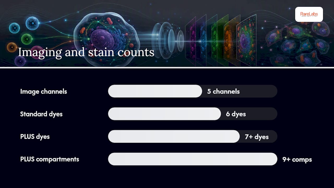
Cell Painting works by multiplexing six fluorescent dyes and imaging them across five channels, which sounds like a compression trick but is really just efficient spectral packing. Two dyes (the ones for cytoplasmic RNA and F-actin, and the Golgi/plasma membrane markers) get imaged in the same channel because their targets rarely overlap in the frame, freeing up bandwidth for the other four independent channels.
Those six dyes collectively illuminate eight compartments: DNA in the nucleus, the endoplasmic reticulum, nucleoli and cytoplasmic RNA, the actin cytoskeleton, the Golgi apparatus, the plasma membrane, mitochondria, and the broader cytoplasm. Each compartment behaves differently under different perturbations. A compound that disrupts microtubule dynamics leaves a very different signature in the actin channel than one that triggers ER stress, and that's the entire premise the assay rests on.
From those images, software extracts features grouped into a handful of categories. Here's what a representative breakdown looks like:
| Feature category | What it captures | Example metric |
|---|---|---|
| Size and shape | Cell and organelle geometry | Nucleus area, cell eccentricity |
| Intensity | Stain signal strength per compartment | Mean mitochondrial intensity |
| Texture | Local pixel pattern complexity | Haralick texture of ER channel |
| Granularity | Fine-grained structure within a compartment | Golgi granularity spectrum |
| Radial distribution | How signal is distributed from center to edge | Actin radial intensity profile |
| Neighbor relationships | Spatial context relative to adjacent cells | Number of touching neighbors |
A single well can generate feature vectors for thousands of individual cells, and that per-cell resolution is what separates Cell Painting from a bulk plate reader assay. You're not averaging a population response. You're capturing a distribution, which matters enormously when a compound only affects a subpopulation of cells or produces heterogeneous responses.
One distinction worth nailing down early: Cell Painting is the assay, not the application. High-content screening (HCS) is the broader category of image-based, multi-parametric screening approaches that Cell Painting operates within. You can run HCS without Cell Painting (a single-marker assay imaged at scale still counts), but you generally can't run Cell Painting without HCS infrastructure, because the data volume and per-cell analysis demand automated imaging and computational pipelines.
Why does morphology reveal mechanism at all? Because most drugs and genetic perturbations don't act on an isolated pathway in isolation. They ripple outward. A kinase inhibitor might primarily hit its target, but downstream effects on cytoskeletal organization, mitochondrial mass, or ER morphology show up as measurable, reproducible shifts. Comparing those shifts across thousands of known compounds lets you infer mechanism for an unknown one by matching its morphological fingerprint.
Cell Painting Protocol: A Stepwise Workflow
A working Cell Painting protocol has six sequential stages, and skipping quality checks at any one of them tends to show up as noise three weeks later during analysis, which is the worst possible time to find it.
- Cell model selection and plating. Choose a cell line or patient-derived model appropriate to your biological question, and plate at a density that yields confluent but non-overlapping cells at imaging time, typically 60 to 80 percent confluency depending on cell type. Use 384-well or 96-well imaging-grade plates with optically clear, flat bottoms.
- Perturbation and treatment timing. Apply compounds, ASOs, or genetic perturbations at a defined time point, then incubate for a fixed window (commonly 24 to 48 hours) before fixation. Consistency in treatment duration matters more than the specific duration you pick.
- Fixation and permeabilization. Fix cells with paraformaldehyde, then permeabilize to allow intracellular dye access. Live-cell compatible variants exist for labs that need to track the same cells over time before endpoint staining, though they trade off some dye options.
- Multiplexed staining. Apply the six-dye cocktail in a defined sequence with wash steps between stages to prevent cross-reactivity, then mount for imaging.
- Imaging acquisition. Image each well across all five channels in a fixed acquisition order, typically DNA first (fastest to focus on) and mitochondria last, capturing multiple fields per well.
- Storage and initial QC. Archive raw images with full metadata, then run a first-pass QC to catch focus failures, illumination artifacts, or missing wells before committing to full feature extraction.
For a batch of 20 plates or fewer, expect culture through imaging to take one to two weeks, with another one to two weeks for feature extraction and initial analysis. Larger screens obviously stretch that timeline, and imaging throughput becomes the bottleneck well before wet-lab capacity does.
Pro Tip: Choose plate types before you finalize your staining protocol, not after. Glass-bottom plates give sharper images at high magnification but cost more and are more fragile in automated handling; polymer-bottom imaging plates are cheaper and robot-friendly but can introduce slight autofluorescence in the blue channel that gets mistaken for real signal. Run a blank-well autofluorescence check with your actual plate lot before you commit to a full screen.
Two variations are worth knowing about even if you don't use them immediately. Live-cell compatible Cell Painting swaps fixable dyes for live-compatible equivalents, useful when you need to track morphological change over time in the same cells rather than a fixed endpoint. And Cell Painting PLUS extends the standard protocol through iterative staining and elution cycles, pushing past eight compartments to nine or more using seven or more dyes total. That extra resolution helps in deep mechanism-of-action or toxicology work, but the iterative cycles roughly double processing time, so reserve it for projects where the standard panel genuinely isn't enough.
Key Stains and Reagents for Cell Painting
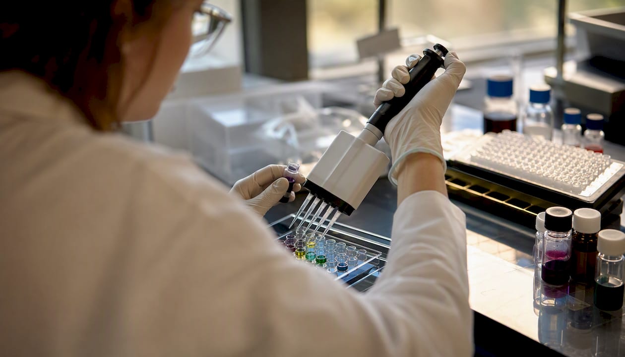
The standard Cell Painting panel uses six specific stains, and while equivalent products exist across vendors, the published concentrations and timings matter more than which brand's bottle you're pipetting from. Dye equivalence across vendors has been validated in v3 testing, meaning strict brand loyalty isn't the reproducibility lever you might assume it is.
| Stain | Target compartment | Typical channel | Practical notes |
|---|---|---|---|
| Hoechst | Nucleus (DNA) | Blue/DAPI | v3 reduced concentration versus original protocol |
| Concanavalin A | Endoplasmic reticulum | Green | Sensitive to fixation timing |
| SYTO | Nucleoli and cytoplasmic RNA | Green (shared) | Co-imaged with actin channel |
| Phalloidin | F-actin cytoskeleton | Red | Binds tightly; wash steps critical |
| Wheat germ agglutinin (WGA) | Golgi and plasma membrane | Red (shared) | Watch for membrane over-saturation |
| MitoTracker | Mitochondria | Far-red | Time-sensitive; add close to imaging |
The 2016 Nature Protocols paper laid out the original concentrations and imaging channel assignments, and the 2023 v3 update in Nature Protocols reduced several stain concentrations and simplified staining steps, cutting reagent cost while preserving phenotype detection performance. If you're setting up a new lab, start from the v3 concentrations rather than the original 2016 values.
On sourcing, a few things worth knowing:
- Commercial kits, including the Thermo Fisher Image-iT Cell Painting Kit, bundle all six dyes in pre-validated ratios, trading flexibility for convenience and reduced pipetting error.
- Buying dyes individually costs less per plate at scale but demands more careful validation of your own working concentrations.
- Cross-talk between co-imaged dyes (RNA/actin and Golgi/membrane) is the most common source of feature noise, so validate your channel assignments with single-stain control wells before running a full plate.
- Fixation reagent choice (typically paraformaldehyde concentration and timing) affects ER and Golgi staining quality more than any other step in the protocol.
Vendor loyalty matters far less than protocol fidelity here. A lab that carefully follows published concentrations with a generic reagent will get more reproducible data than one that uses a premium kit but drifts from validated timing.
Imaging Setup and Throughput for High-Content Screening
Instrument choice shapes everything downstream, from segmentation accuracy to how many plates you can realistically process in a week. Three broad instrument classes dominate Cell Painting work: wide-field epifluorescence microscopes, confocal or spinning-disk systems, and dedicated high-content imaging platforms built specifically for automated plate-based acquisition.
Wide-field systems are the cheapest entry point and work fine for many Cell Painting applications, but they sacrifice some resolution and signal-to-noise ratio compared to confocal alternatives, particularly in thicker or more crowded cell layers. Confocal and spinning-disk systems improve optical sectioning and reduce out-of-focus blur, at the cost of slower acquisition per field. Dedicated high-content platforms, the category Molecular Devices instruments and similar systems occupy, are purpose-built for exactly this workflow: automated plate handling, multi-channel acquisition, and integrated analysis software designed around image-based profiling rather than retrofitted onto general microscopy.
A handful of acquisition parameters determine whether your images are actually usable for downstream feature extraction, and you should record every one of them as metadata:
- Objective numerical aperture and magnification (20x is common for Cell Painting; higher magnification trades field size for resolution).
- Exposure time per channel, tuned to avoid saturation without underexposing dimmer stains.
- Camera bit depth, generally 16-bit for adequate dynamic range across intensity features.
- Pixel size, which determines the smallest morphological feature you can reliably resolve.
- Z-plane strategy: single focal plane versus a z-stack, depending on whether your cell model is flat or three-dimensional.
- Number of fields imaged per well, balancing statistical power against acquisition time.
Throughput trade-offs are real and worth planning around before you start rather than discovering mid-screen. A higher magnification objective gives better morphological resolution but fewer cells per field, meaning more fields needed per well to hit adequate cell counts, which slows plate-per-day throughput. For batches of 20 plates or fewer, this rarely matters much. For large screens pushing into the hundreds of plates, camera speed and fields-per-well decisions can be the difference between a two-week screen and a two-month one.
Pro Tip: Run an illumination uniformity check across the full plate before every imaging session, not just at setup. Uneven illumination introduces a systematic bias that looks like biological signal in edge wells versus center wells, and it's one of the most common causes of spurious plate-position effects in Cell Painting data.
Before trusting a full plate's worth of images, run these checks:
- Focus metrics across representative wells, flagging any with blur scores outside your normal range.
- Illumination profile uniformity across the plate, not just a single reference well.
- Channel bleed-through tests using single-stain controls to confirm each channel captures only its intended dye.
- Spot-check a subset of wells visually before committing the full plate to automated feature extraction.
A multi-site assessment across imaging systems found that different microscopes and acquisition settings materially change assay performance metrics, which reinforces why instrument-specific QC and normalization aren't optional steps you can skip to save time. If you're comparing data collected on two different instruments, expect to normalize for instrument-specific batch effects before any cross-comparison means anything.
From Images to Data: The Cell Painting Analysis Pipeline
Raw images become usable morphological signatures through a modular pipeline: preprocessing and QC, segmentation, feature extraction, aggregation and normalization, then batch correction. Each stage has failure modes that propagate downstream if you don't catch them early.
Preprocessing handles illumination correction and flags obviously corrupted images before they enter the pipeline. Segmentation identifies individual nuclei and cell boundaries, typically nucleus-first since Hoechst staining gives the cleanest boundaries, then expanding outward to define whole-cell regions. Feature extraction then measures intensity, texture, granularity, radial distribution, and shape across every segmented cell, producing the raw feature table. Per-cell values get aggregated to well-level or treatment-level summaries, normalized against plate controls, and finally corrected for batch effects introduced by plate, day, or imaging session.
CellProfiler, maintained by the Broad Institute, remains the standard open-source tool for the classical pipeline, offering modular segmentation and feature extraction steps that most published Cell Painting studies build on. Beyond classical features, deep-learning approaches like DeepProfiler and emerging Vision Transformer or DINO-based representation learning methods extract learned embeddings directly from images rather than hand-engineered features.
| Approach | Strength | Trade-off |
|---|---|---|
| Classical (CellProfiler) | Interpretable, well-validated, transparent features | Requires careful pipeline tuning per cell type |
| Deep learning (DeepProfiler, CNNs) | Captures subtle patterns humans wouldn't design features for | Less interpretable; needs more compute and data |
| Vision Transformer / DINO approaches | Strong performance on large, diverse datasets | Emerging; less established validation history |
Recent literature reports deep learning representations improving chemical perturbation classification by meaningful margins over classical feature extraction in certain benchmarks. That doesn't mean classical features are obsolete. For smaller datasets or projects where interpretability matters, like explaining to a physician-scientist collaborator why two compounds cluster together, classical features remain the more defensible choice. Deep learning representations tend to pay off most clearly at larger dataset scale, where there's enough data for the model to learn genuinely useful structure rather than overfitting to instrument-specific noise.
A few data engineering notes that save real pain later: budget for tens of terabytes of image storage on any screen beyond a pilot scale, since raw image volumes accumulate faster than most teams anticipate. Preserve full metadata (plate ID, well position, acquisition date, instrument, reagent lot) alongside every feature table, and build a reproducible experiment manifest so a collaborator can reconstruct exactly how a given dataset was generated six months later.
Pro Tip: Build percent-replicating and percent-matching metrics into your pipeline from the very first pilot plate, not after you've scaled up. These metrics compare replicate wells against each other and against known reference compounds, and they're the fastest way to catch a broken assay before you've burned a month of imaging time on it.
Designing Robust Cell Painting Experiments
Plate layout decisions made before you plate a single well determine whether your data is trustworthy months later. Randomize compound placement across the plate rather than grouping by treatment class, since systematic row or column effects (from uneven incubator temperature, edge evaporation, or pipetting order) will otherwise masquerade as biological signal. Include both positive controls (compounds with a well-characterized morphological effect) and negative controls (vehicle-only wells) on every plate, not just once per experiment.
Replicate structure needs to work at two levels: intra-plate replicates (the same treatment appearing in multiple wells on one plate) and inter-plate replicates (the same treatment repeated across separate plates run on different days). Intra-plate replicates catch pipetting and edge-well artifacts; inter-plate replicates catch day-to-day and batch-level drift. Skimping on either leaves you unable to distinguish a real hit from a mundane systematic artifact.
Common failure modes and how to work through them:
- Poor or inconsistent staining. Check dye lot age first, then verify fixation timing before assuming a biological cause.
- Uneven illumination. Re-run the illumination uniformity check; if it fails, recalibrate before continuing rather than trying to correct for it computationally after the fact.
- Segmentation errors. Inspect a random sample of segmented images visually; adjust nucleus-detection thresholds before touching whole-cell boundary parameters.
- Dye cross-talk. Rerun single-stain control wells to isolate which channel pair is bleeding into the other, then adjust exposure times or filter sets.
- Edge effects. Compare center-well versus edge-well control values directly; if they differ significantly, consider excluding outer wells or improving plate sealing.
- Fixation artifacts. Shortened or extended fixation windows show up as ER and Golgi staining irregularities first, so troubleshoot those channels before others.
- Cell clumping. Reduce plating density and revisit trypsinization technique before changing anything downstream in imaging or analysis.
Before committing to a full-scale screen, run a pilot and evaluate it against two key metrics: percent replicating (how consistently replicate wells of the same treatment cluster together) and an image-based adaptation of the classic Z′ statistic used to judge whether positive and negative controls are cleanly separable. A pilot that fails either metric needs troubleshooting before scaling, not after. This is also where validating your cellular disease model upfront pays real dividends, since a poorly characterized cell model will produce ambiguous Cell Painting signatures no matter how clean your imaging is.
Where Cell Painting Assays Deliver the Most Value
Five use cases account for most of the published Cell Painting literature: mechanism-of-action deconvolution for unknown compounds, toxicity and hazard screening ahead of more expensive downstream studies, compound clustering and hit triage in early discovery, genetic perturbation phenotyping (CRISPR knockouts or knockdowns compared against wild type), and integrative analyses that combine morphological profiles with transcriptomic or proteomic data, highlighting why cell assays are important for drug discovery.
The clustering application is where the assay's value becomes most tangible. Compounds sharing a mechanism of action tend to produce similar morphological fingerprints even when their chemical structures look nothing alike, letting researchers group an unknown compound with known reference compounds based purely on phenotypic similarity. This kind of guilt-by-association reasoning has repeatedly surfaced mechanism hypotheses that single-endpoint assays would have missed entirely, because those assays only measure the one pathway you thought to test.
The real power of Cell Painting isn't any individual feature. It's the high-dimensional morphological signature as a whole, which lets you computationally compare thousands of perturbations against each other and surface mechanistic relationships that no single biochemical readout would ever reveal.
Public datasets and image galleries from the Broad Institute and the JUMP-CP consortium give researchers a way to inspect real Cell Painting images and profiles before committing to their own pilot, which is worth doing if you've never seen raw output from this assay before. Seeing what a genuinely clean mitochondrial channel looks like, versus one with early photobleaching, saves a lot of guesswork later. For labs weighing whether phenotypic screening fits their broader discovery strategy, it's worth reviewing drug screening approaches for biopharma research alongside Cell Painting specifically, since the assay tends to work best as one component of a larger screening funnel rather than a standalone decision tool.
Applying Cell Painting to Rare-Disease Modeling
Patient-derived induced pluripotent stem cells (iPSCs), differentiated into a disease-relevant cell type and paired with a CRISPR-edited isogenic control, give Cell Painting something most drug discovery programs never get: a direct, cell-level comparison between a specific patient's disease state and a genetically matched normal control. Any morphological difference that shows up between the two isn't confounded by genetic background variation, since the isogenic control differs from the patient line at exactly the edited locus and nowhere else.
That matters enormously for ultra-rare diseases, where you typically have one patient, or at most a handful, rather than the hundreds needed for traditional population-scale statistics. Cell Painting's per-cell resolution partly compensates for small sample size. A single well can generate morphological data from thousands of individual cells, and that per-cell statistical power lets you detect a real phenotypic difference between disease and control lines even when you can't run the large cohort a typical clinical study would need.
Practical design notes for a small-n rare-disease project:
- Run more replicate wells per condition than you would in a standard compound screen, since you're compensating for having only one or two patient lines rather than a diverse compound library.
- Lean on public reference datasets from the JUMP-CP consortium to contextualize how large a morphological shift needs to be before it's likely meaningful, rather than guessing at a threshold from scratch.
- Prioritize positive controls with well-characterized effects on the specific compartments you expect the disease biology to touch, rather than generic reference compounds.
- Pair the isogenic control comparison with a second orthogonal assay (a transcriptomic readout or a functional assay specific to the disease biology) to validate that a morphological hit reflects real biology rather than clonal variation from the iPSC line itself.
Pro Tip: Once you've established a disease-versus-control morphological signature, screen it against a library of FDA-approved drugs and custom antisense oligonucleotides rather than a generic compound collection first. Repurposed drugs come with existing safety data, which meaningfully shortens the path from a Cell Painting hit to something a physician can actually consider for a patient. Screening FDA-approved drug libraries against a validated morphological signature is precisely the kind of translational step that makes personalized modeling actionable rather than purely academic, and it connects directly to why rapid screening matters so much for rare disease families facing a narrow treatment window.
Where to Find the Protocols, Datasets, and Tools
Three types of resources matter here, and they answer different questions. For protocol details, the original Bray et al. 2016 Nature Protocols paper remains the canonical citation for staining steps and reagent concentrations, while the 2023 v3 update gives the current optimized concentrations most new labs should start from.
For analysis pipelines, CellProfiler from the Broad Institute is the open-source standard for classical feature extraction, with published pipelines available for direct adaptation. DeepProfiler and related deep-learning repositories offer an alternative path for teams with larger datasets and computational infrastructure already in place.
For datasets and community benchmarking, the JUMP-Cell Painting Consortium hosts reference plates and public datasets that let you benchmark your own staining and imaging conditions against a multi-site standard before trusting your first full screen. Public image and profile collections from the Broad Institute give a useful reference point for what typical phenotypic signatures look like across thousands of perturbations, which is worth reviewing before you interpret your own pilot data in isolation.
A quick rule of thumb: consult Bray et al. and the v3 update for wet-lab protocol questions, CellProfiler documentation for analysis pipeline questions, and the JUMP-CP portal for reproducibility benchmarks and public reference data.
What Labs Get Wrong Starting Out
Most first-time Cell Painting projects fail for boring reasons, not exotic ones. The three things worth getting right before you touch a pipette matter more than any advanced technique you might read about later.
Start small, and start with the pilot design questions answered before you plate anything: how many replicate wells, which controls, and what plate layout will you actually use. A 20-plate pilot with careful controls beats a 100-plate screen with sloppy layout every time, because you can't fix a confounded plate design after the fact no matter how good your analysis pipeline is. Second, imaging QC deserves at least as much attention as the wet-lab protocol itself. Teams that treat imaging as a formality tend to discover, weeks later during analysis, that half their plates have a subtle illumination gradient nobody caught in real time.
The choice between classical features and deep-learning embeddings comes down to project goals and dataset size, not which method sounds more impressive. If you're running a focused pilot with a handful of conditions, classical CellProfiler features give you interpretable results you can defend to a collaborator or reviewer. If you're sitting on a large, diverse dataset spanning hundreds of perturbations, deep-learning representations start to earn their computational cost through genuinely better performance on classification tasks.
Reproducibility isn't something you bolt on at the end. Invest in control plates and a batch-correction plan from the very first experiment, because retrofitting normalization onto data you already collected without adequate controls is a much harder problem than designing it in from the start. Teams that treat control-plate design as an afterthought almost always end up re-running experiments they thought were finished.
How Hopeatrarelabs Applies Cell Painting to Rare Disease Programs
If your lab is weighing whether to build Cell Painting capability in-house versus working with a partner who already runs this pipeline daily, the calculation usually comes down to how much time you can dedicate to imaging QC and analysis infrastructure before your actual research question gets answered. Hopeatrarelabs builds patient-specific iPSC and CRISPR-edited isogenic disease models and runs high-throughput repurposed drug screening on them, using morphological profiling as one layer in a broader parallel screen against FDA-approved drugs, custom ASOs, and gene therapy candidates for ultra-rare and undiagnosed genetic diseases.

For families, physicians, and foundations who need translational movement rather than another year of assay optimization, that means the disease modeling, screening, and Cell Painting-informed hit triage happen inside one program instead of being stitched together across separate vendors. If you're a patient, family, foundation, or biopharma partner looking to start a personalized modeling and screening program for a specific rare disease, reach out to Hopeatrarelabs to discuss what a pilot program would look like for your case.
Primary Sources and Recommended Reading
- Bray et al., Cell Painting protocol, PMC: the canonical wet-lab protocol, reagent concentrations, and imaging channel assignments.
- Optimizing the Cell Painting assay, Nature Protocols v3: current recommended stain concentrations and reproducibility improvements.
- JUMP-Cell Painting Consortium: reference plates, public datasets, and cross-site benchmarking resources.
- Cell Painting: a decade of discovery, PMC: a comprehensive review of applications, analysis trends, and QC considerations.
- Assessing Cell Painting performance across imaging systems, bioRxiv: data on how instrument choice affects assay performance and normalization needs.
Consult the Bray et al. protocol and its v3 update for wet-lab implementation questions, the JUMP-CP consortium for reproducibility benchmarks and public data, and the decade-in-review paper for a broader sense of how the field's analysis methods have evolved.
Sources
- Cell Painting, a high-content image-based assay for morphological profiling using multiplexed fluorescent dyes
- Cell Painting: a decade of discovery and innovation in cellular imaging
- Assessing the performance of the Cell Painting assay across different imaging systems